from caml.extensions.synthetic_data import SyntheticDataGenerator

data_generator = SyntheticDataGenerator(
    n_obs=10_000,
    n_cont_outcomes=1,
    n_binary_treatments=1,
    n_cont_confounders=2,
    n_cont_modifiers=2,
    n_confounding_modifiers=1,
    causal_model_functional_form="linear",
    seed=10,
)AutoCATE
In this notebook, we’ll walk through an example of generating synthetic data, running AutoCATE, and visualizing results using the ground truth as reference.
AutoCATE is particularly useful when highly accurate CATE estimation is of primary interest in the presence of exogenous treatment, simple linear confounding, or complex non-linear confounding.
AutoCATE enables the use of various CATE models with varying assumptions on functional form of treatment effects & heterogeneity. When a set of CATE models are considered, the final CATE model is automatically selected based on validation set performance.
🚀Forthcoming: The
AutoCATEclass is in a very experimental, infancy stage. Additional scoring techniques & a more robust AutoML framework for CATE estimators is on our roadmap.
Generate Synthetic Data
Here we’ll leverage the SyntheticDataGenerator class to generate a linear synthetic data generating process, with a binary treatment, continuous outcome, and a mix of confounding/mediating continuous covariates.
We can print our simulated data via:
data_generator.df| W1_continuous | W2_continuous | X1_continuous | X2_continuous | T1_binary | Y1_continuous | |
|---|---|---|---|---|---|---|
| 0 | 0.354380 | -3.252276 | 2.715662 | -3.578800 | 1 | 11.880305 |
| 1 | 0.568499 | 2.484069 | -6.402235 | -2.611815 | 0 | -32.292141 |
| 2 | 0.162715 | 8.842902 | 1.288770 | -3.788545 | 1 | -48.696391 |
| 3 | 0.362944 | -0.959538 | 1.080988 | -3.542550 | 0 | -1.899468 |
| 4 | 0.612101 | 1.417536 | 4.143630 | -4.112453 | 1 | -7.315334 |
| ... | ... | ... | ... | ... | ... | ... |
| 9995 | 0.340436 | 0.241095 | -6.524222 | -3.188783 | 1 | -27.578609 |
| 9996 | 0.019523 | 1.338152 | -2.555492 | -3.643733 | 1 | -19.692436 |
| 9997 | 0.325401 | 1.258659 | -3.340546 | -4.255203 | 1 | -26.087316 |
| 9998 | 0.586715 | 1.263264 | -2.826709 | -4.149383 | 1 | -25.876331 |
| 9999 | 0.003002 | 6.723381 | 1.260782 | -3.660600 | 1 | -38.200522 |
10000 rows × 6 columns
To inspect our true data generating process, we can call data_generator.dgp. Furthermore, we will have our true CATEs and ATEs at our disposal via data_generator.cates & data_generator.ates, respectively. We’ll use this as our source of truth for performance evaluation of our CATE estimator.
for t, df in data_generator.dgp.items():
    print(f"\nDGP for {t}:")
    print(df)
DGP for T1_binary:
{'formula': '1 + W1_continuous + W2_continuous + X1_continuous', 'params': array([ 0.4609703 ,  0.2566887 , -0.03896251,  0.07238272]), 'noise': array([-0.51949108, -1.88624383,  0.86927397, ...,  0.87157749,
        0.0697439 , -0.72616319], shape=(10000,)), 'raw_scores': array([0.58800598, 0.13710535, 0.75412862, ..., 0.7549587 , 0.60527474,
       0.39290362], shape=(10000,)), 'function': <function SyntheticDataGenerator._create_dgp_function.<locals>.f_binary at 0x7f8ce4624a60>}

DGP for Y1_continuous:
{'formula': '1 + W1_continuous + W2_continuous + X1_continuous + X2_continuous + T1_binary + T1_binary*X1_continuous + T1_binary*X2_continuous', 'params': array([ 1.11129512, -4.1263484 , -4.82709212,  1.87319625,  2.60635605,
       -0.91633948,  0.71653213, -0.25067306]), 'noise': array([-1.15370094, -0.26681987,  0.05261899, ..., -0.18887322,
       -0.45736583, -0.57057603], shape=(10000,)), 'raw_scores': array([ 11.88030508, -32.29214063, -48.69639077, ..., -26.0873159 ,
-25.87633114, -38.20052217], shape=(10000,)), 'function': <function SyntheticDataGenerator._create_dgp_function.<locals>.f_cont at 0x7f8c5cd7fbe0>}data_generator.cates| CATE_of_T1_binary_on_Y1_continuous | |
|---|---|
| 0 | 1.926628 |
| 1 | -4.849035 |
| 2 | 0.956792 |
| 3 | 0.746245 |
| 4 | 3.083586 |
| ... | ... |
| 9995 | -4.791812 |
| 9996 | -1.834046 |
| 9997 | -2.243283 |
| 9998 | -1.901629 |
| 9999 | 0.904665 |
10000 rows × 1 columns
data_generator.ates| Treatment | ATE | |
|---|---|---|
| 0 | T1_binary_on_Y1_continuous | -0.55937 |
Running AutoCATE
Class Instantiation
We can instantiate and observe our AutoCATE object via:
Tip
W can be leveraged if we want to use certain covariates only in our nuisance functions to control for confounding and not in the final CATE estimator. This can be useful if a confounder may be required to include, but for compliance reasons, we don’t want our CATE model to leverage this feature (e.g., gender). However, this will restrict our available CATE estimators to orthogonal learners, since metalearners necessarily include all covariates. If you don’t care about W being in the final CATE estimator, pass it as X, as done below.
from caml import AutoCATE

auto_cate = AutoCATE(
    Y="Y1_continuous",
    T="T1_binary",
    X=[c for c in data_generator.df.columns if "X" in c]
    + [c for c in data_generator.df.columns if "W" in c],
    discrete_treatment=True,
    discrete_outcome=False,
    model_Y={
        "time_budget": 10,
        "estimator_list": ["rf", "extra_tree", "xgb_limitdepth"],
    },
    model_T={
        "time_budget": 10,
        "estimator_list": ["rf", "extra_tree", "xgb_limitdepth"],
    },
    model_regression={
        "time_budget": 10,
        "estimator_list": ["rf", "extra_tree", "xgb_limitdepth"],
    },
    enable_categorical=True,
    n_jobs=-1,
    use_ray=False,
    ray_remote_func_options_kwargs=None,
    use_spark=False,
    seed=None,
)
[11/13/25 16:47:54] WARNING AutoCATE is experimental and may change in future versions. decorators.py:47
Fitting End-to-End AutoCATE pipeline
First, I can inspect available estimators out of the box:
auto_cate.available_estimators['LinearDML',
'CausalForestDML',
'NonParamDML',
'SparseLinearDML-2D',
'DRLearner',
'ForestDRLearner',
'LinearDRLearner',
'SLearner',
'TLearner',
'XLearner']And create another one if desired:
from caml import AutoCateEstimator
from econml.dml import LinearDML

my_custom_estimator = AutoCateEstimator(name="MyCustomEstimator",estimator=LinearDML())
auto_cate.fit(data_generator.df, cate_estimators=['LinearDML','CausalForestDML','TLearner'], additional_cate_estimators=[my_custom_estimator])INFO decorators.py:93 ____ __ __ _ / ___|__ _| \/ | | | | / _` | |\/| | | | |__| (_| | | | | |___ \____\__,_|_| |_|_____|
                    INFO     ================== AutoCATE Object ==================                      cate.py:298
                             Outcome Variable: ['Y1_continuous']
                             Discrete Outcome: False
                             Treatment Variable: ['T1_binary']
                             Discrete Treatment: True
                             Features/Confounders for Heterogeneity (X): ['X1_continuous',
                             'X2_continuous', 'W1_continuous', 'W2_continuous']
                             Features/Confounders as Controls (W): []
                             Enable Categorical: True
                             n Jobs: -1
                             Use Ray: False
                             Use Spark: False
                             Random Seed: None
                    INFO                                                                           decorators.py:93
                             ==============================
                             |🎯 AutoML Nuisance Functions|
                             ==============================
[11/13/25 16:48:04] INFO     Best estimator: extra_tree with loss 5.526333452848555 found on iteration _base.py:144
                             36 in 9.822532892227173 seconds.
[11/13/25 16:48:15] INFO     Best estimator: rf with loss 3.537512927034561 found on iteration 28 in   _base.py:144
                             5.735426425933838 seconds.
[11/13/25 16:48:25] INFO     Best estimator: rf with loss 0.6739378405925093 found on iteration 31 in  _base.py:144
                             5.714165210723877 seconds.
INFO ✅ Completed. decorators.py:98
                    INFO                                                                           decorators.py:93
                             ==========================
                             |🎯 AutoML CATE Functions|
                             ==========================
                    INFO     Estimator RScores: {'LinearDML': np.float64(0.36464873416158483),          cate.py:838
                             'CausalForestDML': np.float64(0.35787409320239394), 'TLearner':
                             np.float64(0.32694013018330437), 'MyCustomEstimator':
                             np.float64(0.3662927922121474)}
INFO ✅ Completed. decorators.py:98
                    INFO                                                                           decorators.py:93
                             ====================
                             |🧪 Testing Results|
                             ====================
[11/13/25 16:48:34] INFO     All validation results suggest that the model has found statistically      cate.py:923
                             significant heterogeneity.
                    INFO        treatment  blp_est  blp_se  blp_pval  qini_est  qini_se  qini_pval  \   cate.py:927
                             0          1    1.016   0.042       0.0     1.016    0.053        0.0

                                autoc_est  autoc_se  autoc_pval  cal_r_squared
                             0      2.767     0.156         0.0           0.92
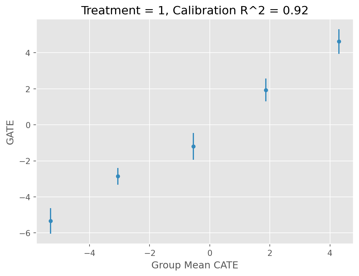
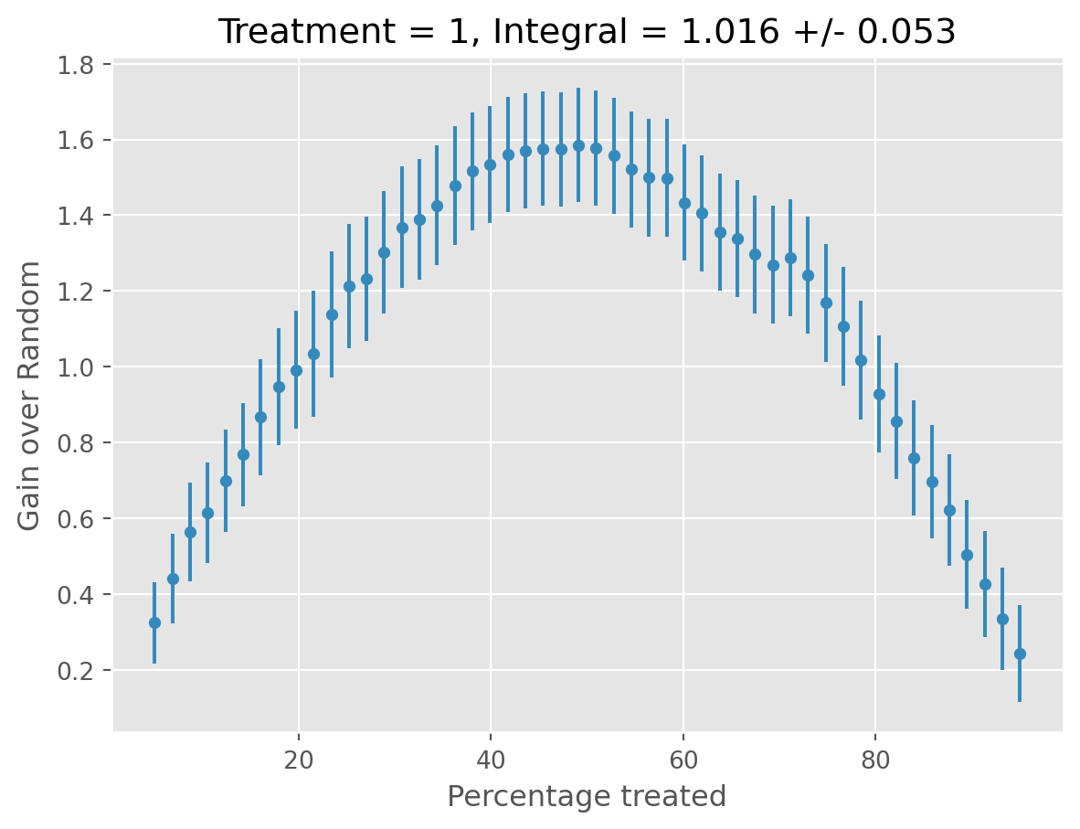
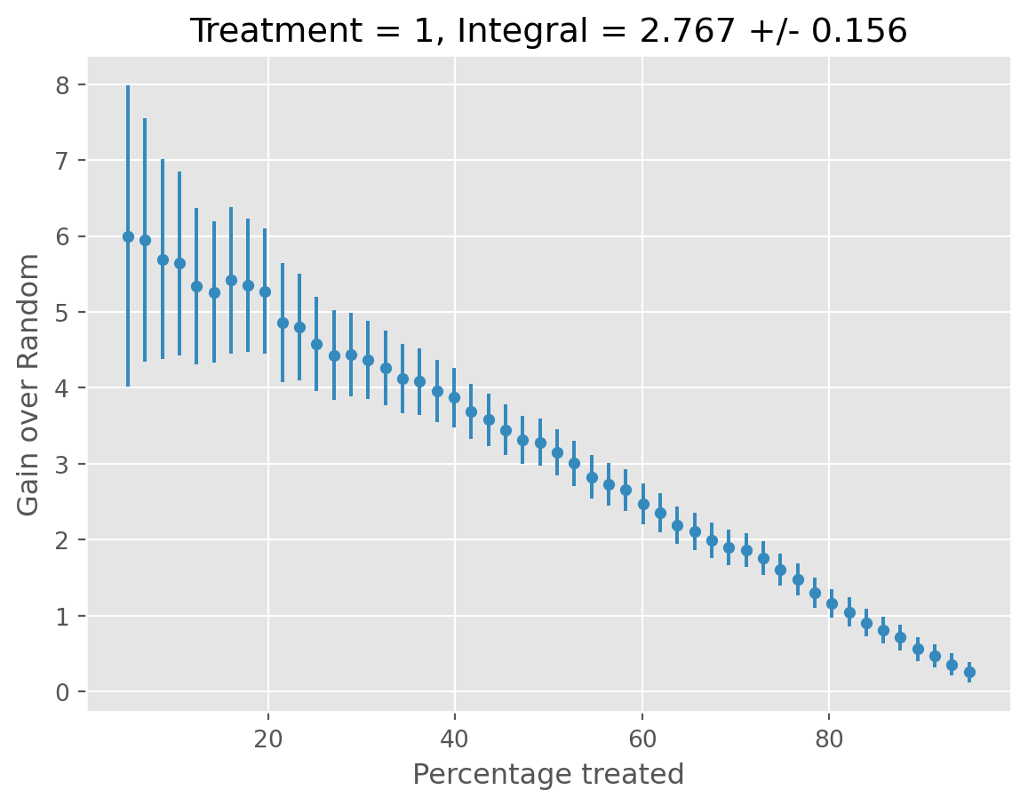
INFO ✅ Completed. decorators.py:98
                    INFO                                                                           decorators.py:93
                             ==============================
                             |🔋 Refitting Final Estimator|
                             ==============================
[11/13/25 16:48:35] INFO ✅ Completed. decorators.py:98
Note
The selected CATE model defaults to the one with the highest RScore.
Validating Results with Ground Truth
Average Treatment Effect (ATE)
We’ll use the summarize() method after obtaining our predictions above, where our the displayed mean represents our Average Treatment Effect (ATE).
auto_cate.estimate_ate(data_generator.df[auto_cate.X])np.float64(-0.5699974339674273)Now comparing this to our ground truth, we see the model performed well the true ATE:
data_generator.ates| Treatment | ATE | |
|---|---|---|
| 0 | T1_binary_on_Y1_continuous | -0.55937 |
Conditional Average Treatment Effect (CATE)
Now we want to see how the estimator performed in modeling the true CATEs.
First, we can simply compute the Precision in Estimating Heterogeneous Effects (PEHE), which is simply the Root Mean Squared Error (RMSE):
from sklearn.metrics import root_mean_squared_error

cate_predictions = auto_cate.estimate_cate(
    data_generator.df[auto_cate.X]
)  # `predict` and `effect` are aliases
true_cates = data_generator.cates.to_numpy()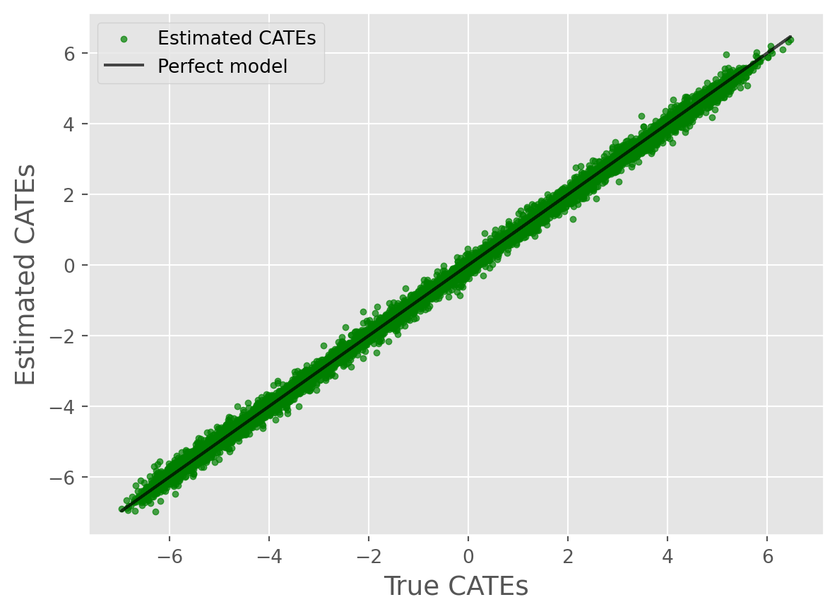
root_mean_squared_error(true_cates, cate_predictions)0.13879792930986268Not bad! Now let’s use some visualization techniques:
from caml.extensions.plots import cate_true_vs_estimated_plot

cate_true_vs_estimated_plot(
    true_cates=true_cates, estimated_cates=cate_predictions
)
from caml.extensions.plots import cate_histogram_plot

cate_histogram_plot(true_cates=true_cates, estimated_cates=cate_predictions)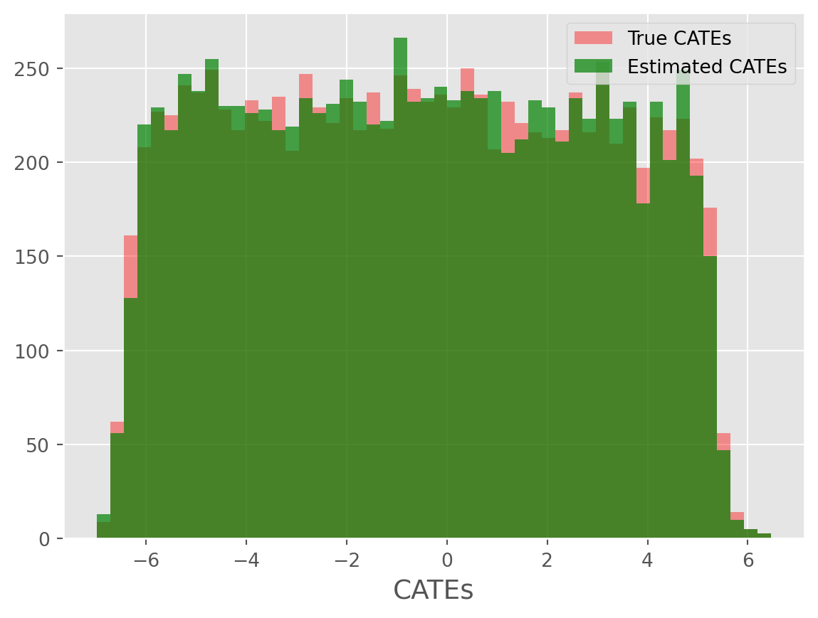
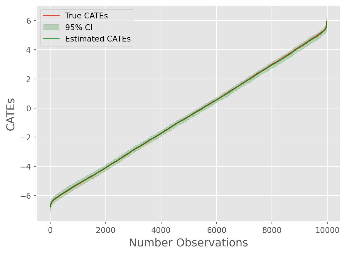
from caml.extensions.plots import cate_line_plot

cate_line_plot(
    true_cates=true_cates.flatten(),
    estimated_cates=cate_predictions.flatten(),
    window=20,
)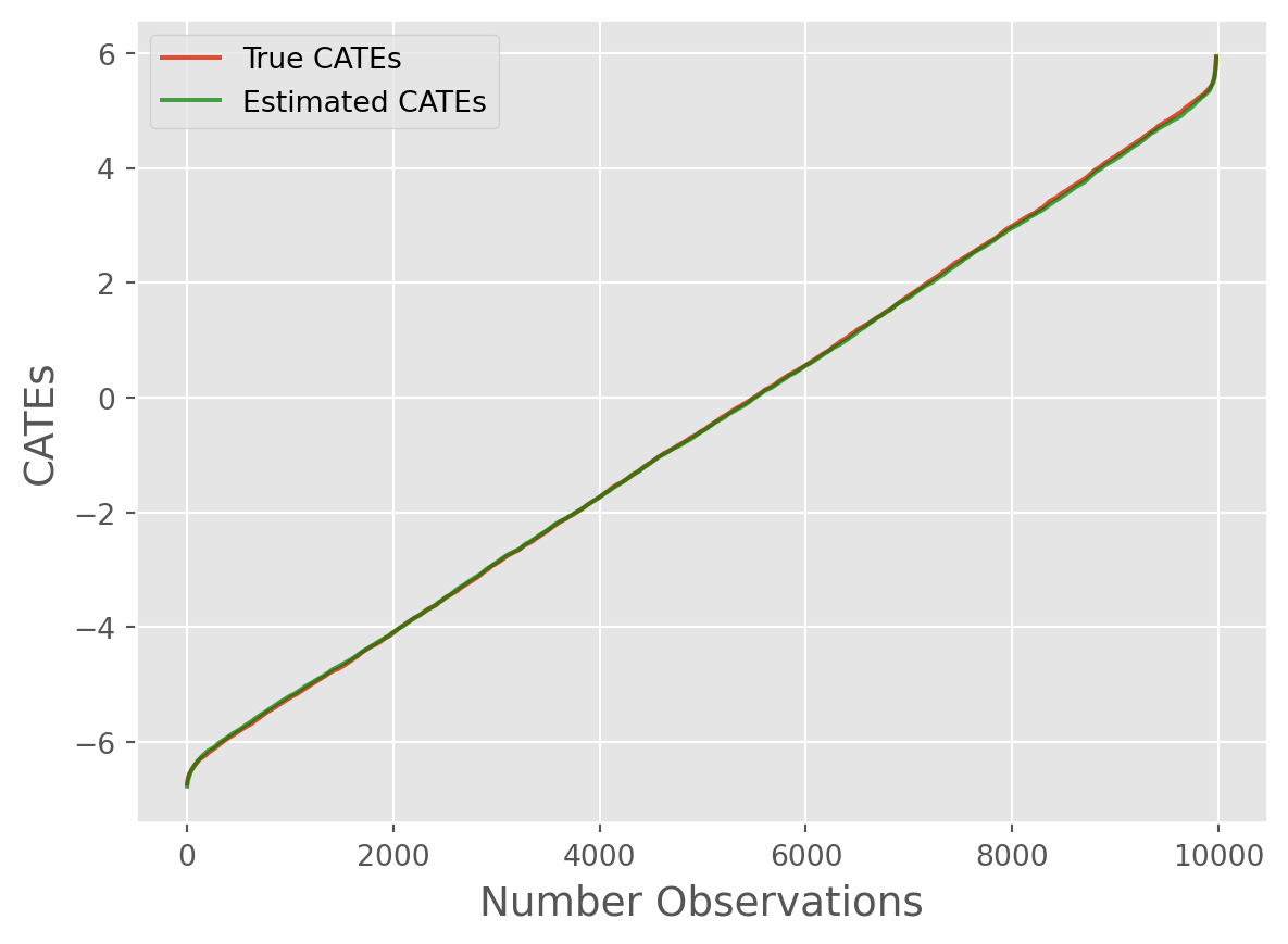
Overall, we can see the model performed remarkably well!
Now, we can also get standard errors by obtaining the EconML Inference Results by passing return_inference=True to estimate_cate (or predict or effect):
inference = auto_cate.estimate_cate(
    data_generator.df[auto_cate.X], return_inference=True
)
stderrs = inference.stderr

cate_line_plot(
    true_cates=true_cates.flatten(),
    estimated_cates=cate_predictions.flatten(),
    window=20,
    standard_errors=stderrs,
)