from caml.logging import configure_logging
import logging

configure_logging(level=logging.DEBUG)
[06/10/25 15:22:53] DEBUG Logging configured with level: DEBUG logging.py:70
In this notebook, we’ll walk through an example of generating synthetic data, estimating treatment effects (ATEs, GATEs, and CATEs) using FastOLS, and comparing to our ground truth.
FastOLS is particularly useful when efficiently estimating ATEs and GATEs is of primary interest and the treatment is exogenous or confounding takes on a particularly simple functional form.
FastOLS assumes linear treatment effects & heterogeneity. This is generally sufficient for estimation of ATEs and GATEs, but can perform poorly in CATE estimation & prediction when heterogeneity is complex & nonlinear. For high quality CATE estimation, we recommend leveraging CamlCATE.
Here we’ll leverage the SyntheticDataGenerator class to generate a linear synthetic data generating process, with an exogenous binary treatment, a continuous & a binary outcome, and binary & continuous mediating covariates.
from caml.logging import configure_logging
import logging
configure_logging(level=logging.DEBUG)[06/10/25 15:22:53] DEBUG Logging configured with level: DEBUG logging.py:70
from caml.extensions.synthetic_data import SyntheticDataGenerator

data_generator = SyntheticDataGenerator(
    n_obs=10_000,
    n_cont_outcomes=1,
    n_binary_outcomes=1,
    n_binary_treatments=1,
    n_cont_confounders=2,
    n_cont_modifiers=3,
    n_binary_modifiers=2,
    stddev_outcome_noise=1,
    stddev_treatment_noise=1,
    causal_model_functional_form="linear",
    seed=10,
)
[06/10/25 15:22:54] WARNING SyntheticDataGenerator is experimental and may change in future generics.py:44 versions.
We can print our simulated data via:
data_generator.df| W1_continuous | W2_continuous | X1_continuous | X2_continuous | X3_continuous | X4_binary | X5_binary | T1_binary | Y1_continuous | Y2_binary | |
|---|---|---|---|---|---|---|---|---|---|---|
| 0 | 0.354380 | -3.252276 | 2.715662 | -3.578800 | -3.148647 | 0 | 0 | 1 | -11.319410 | 0 |
| 1 | 0.568499 | 2.484069 | -6.402235 | -2.611815 | -0.311498 | 0 | 0 | 1 | 9.167825 | 1 |
| 2 | 0.162715 | 8.842902 | 1.288770 | -3.788545 | -1.780285 | 0 | 0 | 0 | -21.010316 | 0 |
| 3 | 0.362944 | -0.959538 | 1.080988 | -3.542550 | -5.419263 | 1 | 0 | 1 | -2.194239 | 0 |
| 4 | 0.612101 | 1.417536 | 4.143630 | -4.112453 | -4.551051 | 0 | 0 | 1 | -20.600668 | 1 |
| ... | ... | ... | ... | ... | ... | ... | ... | ... | ... | ... |
| 9995 | 0.340436 | 0.241095 | -6.524222 | -3.188783 | -2.313515 | 0 | 0 | 1 | 16.349832 | 1 |
| 9996 | 0.019523 | 1.338152 | -2.555492 | -3.643733 | -5.517065 | 0 | 1 | 1 | 5.386195 | 1 |
| 9997 | 0.325401 | 1.258659 | -3.340546 | -4.255203 | -2.272974 | 0 | 0 | 1 | -1.037638 | 0 |
| 9998 | 0.586715 | 1.263264 | -2.826709 | -4.149383 | -2.712932 | 0 | 0 | 1 | -0.235958 | 1 |
| 9999 | 0.003002 | 6.723381 | 1.260782 | -3.660600 | -0.962271 | 0 | 0 | 0 | -20.007912 | 1 |
10000 rows × 10 columns
To inspect our true data generating process, we can call data_generator.dgp. Furthermore, we will have our true CATEs and ATEs at our disposal via data_generator.cates & data_generator.ates, respectively. We’ll use this as our source of truth for performance evaluation of our CATE estimator.
for t, df in data_generator.dgp.items():
    print(f"\nDGP for {t}:")
    print(df)
DGP for T1_binary:
{'formula': '1 + W1_continuous + W2_continuous', 'params': array([0.00323235, 0.14809798, 0.00393589]), 'noise': array([ 0.41708078,  2.72097405, -0.05882655, ...,  0.53984804,
        1.50464572, -0.08231107]), 'raw_scores': array([0.6130131 , 0.9436502 , 0.50082704, ..., 0.6447923 , 0.83198225,
       0.48696005]), 'function': <function SyntheticDataGenerator._create_dgp_function.<locals>.f_binary at 0x7f88407cf2e0>}

DGP for Y1_continuous:
{'formula': '1 + W1_continuous + W2_continuous + X1_continuous + X2_continuous + X3_continuous + X4_binary + X5_binary + T1_binary + T1_binary*X1_continuous + T1_binary*X2_continuous + T1_binary*X3_continuous + T1_binary*X4_binary + T1_binary*X5_binary', 'params': array([-0.35986539, -3.30656481, -1.08522702, -2.03156347,  4.15748518,
       -3.7649075 ,  2.0412171 , -4.06259065,  1.19724956, -1.49108621,
       -0.33216768,  1.0519125 , -0.68252501,  0.57505328]), 'noise': array([ 0.19963494, -0.500903  ,  1.15056187, ..., -1.08977141,
        0.79262583,  1.81566293]), 'raw_scores': array([-11.31940995,   9.16782505, -21.01031565, ...,  -1.03763754,
        -0.23595847, -20.00791171]), 'function': <function SyntheticDataGenerator._create_dgp_function.<locals>.f_cont at 0x7f88407cf7f0>}

DGP for Y2_binary:
{'formula': '1 + W1_continuous + W2_continuous + X1_continuous + X2_continuous + X3_continuous + X4_binary + X5_binary + T1_binary + T1_binary*X1_continuous + T1_binary*X2_continuous + T1_binary*X3_continuous + T1_binary*X4_binary + T1_binary*X5_binary', 'params': array([-0.69301323,  0.54152509,  0.39837891,  0.15335688,  0.39980853,
       -0.31388112, -0.18490127,  0.25395436,  0.19802621, -0.84703988,
       -0.12066193,  0.09225998,  0.37205785, -0.20954318]), 'noise': array([ 1.07352996,  0.43383419, -1.01413765, ..., -1.15478882,
        0.58572912,  0.22523345]), 'raw_scores': array([0.06237408, 0.99      , 0.75869455, ..., 0.65949716, 0.91015409,
0.77628529]), 'function': <function SyntheticDataGenerator._create_dgp_function.<locals>.f_binary at 0x7f88407e5d80>}data_generator.cates| CATE_of_T1_binary_on_Y1_continuous | CATE_of_T1_binary_on_Y2_binary | |
|---|---|---|
| 0 | -4.975376 | -0.116864 |
| 1 | 11.283425 | 0.779704 |
| 2 | -1.338690 | -0.070368 |
| 3 | -5.620992 | -0.088495 |
| 4 | -8.402543 | -0.582547 |
| ... | ... | ... |
| 9995 | 9.551022 | 0.857542 |
| 9996 | 0.989622 | 0.391185 |
| 9997 | 5.200762 | 0.679941 |
| 9998 | 3.936641 | 0.602064 |
| 9999 | -0.478977 | -0.111850 |
10000 rows × 2 columns
data_generator.ates| Treatment | ATE | |
|---|---|---|
| 0 | T1_binary_on_Y1_continuous | 1.195965 |
| 1 | T1_binary_on_Y2_binary | 0.152762 |
We can instantiate and observe our FastOLS object via:
from caml import FastOLS

fo_obj = FastOLS(
    Y=[c for c in data_generator.df.columns if "Y" in c],
    T="T1_binary",
    G=[
        c
        for c in data_generator.df.columns
        if "X" in c and ("bin" in c or "dis" in c)
    ],
    X=[c for c in data_generator.df.columns if "X" in c and "cont" in c],
    W=[c for c in data_generator.df.columns if "W" in c],
    xformula="+ W1_continuous**2",
    engine="cpu",
    discrete_treatment=True,
)
WARNING FastOLS is experimental and may change in future versions. generics.py:44
                    DEBUG    Initializing FastOLS with parameters: Y=['Y1_continuous', 'Y2_binary'],     ols.py:146
                             T=T1_binary, G=['X4_binary', 'X5_binary'], X=['X1_continuous',
                             'X2_continuous', 'X3_continuous'], W=['W1_continuous', 'W2_continuous'],
                             discrete_treatment=True, engine=cpu
                    DEBUG    Created formula: Q('Y1_continuous') + Q('Y2_binary') ~ C(Q('T1_binary')) +  ols.py:177
                             C(Q('X4_binary'))*C(Q('T1_binary')) + C(Q('X5_binary'))*C(Q('T1_binary')) +
                             Q('X1_continuous')*C(Q('T1_binary')) + Q('X2_continuous')*C(Q('T1_binary'))
                             + Q('X3_continuous')*C(Q('T1_binary')) + Q('W1_continuous') +
                             Q('W2_continuous') + W1_continuous**2
print(fo_obj)================== FastOLS Object ==================
Engine: cpu
Outcome Variable: ['Y1_continuous', 'Y2_binary']
Treatment Variable: T1_binary
Discrete Treatment: True
Group Variables: ['X4_binary', 'X5_binary']
Features/Confounders for Heterogeneity (X): ['X1_continuous', 'X2_continuous', 'X3_continuous']
Features/Confounders as Controls (W): ['W1_continuous', 'W2_continuous']
Formula: Q('Y1_continuous') + Q('Y2_binary') ~ C(Q('T1_binary')) + C(Q('X4_binary'))*C(Q('T1_binary')) + C(Q('X5_binary'))*C(Q('T1_binary')) + Q('X1_continuous')*C(Q('T1_binary')) + Q('X2_continuous')*C(Q('T1_binary')) + Q('X3_continuous')*C(Q('T1_binary')) + Q('W1_continuous') + Q('W2_continuous') + W1_continuous**2
We can now leverage the fit method to estimate the model outlined by fo_obj.formula. To capitalize on efficiency gains and parallelization in the estimation of GATEs, we will pass estimate_effects=True. The n_jobs argument will control the number of parallel jobs (GATE estimations) executed at a time. We will set n_jobs=-1 to use all available cores for parallelization.
When dealing with large datasets, setting n_jobs to a more conservative value can help prevent OOM errors.
For heteroskedasticity-robust variance estimation, we will also pass robust_vcv=True.
fo_obj.fit(
    data_generator.df, n_jobs=-1, estimate_effects=True, cov_type="HC1"
)
DEBUG Design Matrix Creation completed in 0.06 seconds generics.py:73
DEBUG Model Fitting completed in 0.02 seconds generics.py:73
DEBUG Design Matrix Creation completed in 0.12 seconds generics.py:73
DEBUG ATE Estimation completed in 0.00 seconds generics.py:73
DEBUG Prespecified GATE Estimation completed in 0.02 seconds generics.py:73
We can now inspect the model fitted results and estimated treatment effects:
fo_obj.params
# fo_obj.vcv
# fo_obj.std_err
# fo_obj.fitted_values
# fo_obj.residuals
array([[-0.4519221 , 0.43114593],
[ 1.38073585, -0.0744549 ],
[ 2.00450453, -0.01259566],
[-4.04210602, 0.02437893],
[-0.65283268, 0.04810221],
[ 0.49183752, -0.01360602],
[-2.02552124, 0.02571064],
[-1.49027655, -0.10135024],
[ 4.14289136, 0.06712511],
[-0.28916188, -0.05434839],
[-3.76790351, -0.05556488],
[ 1.05912299, 0.03298887],
[-1.63464173, 0.03581225],
[-1.07407314, 0.04467536],
[-1.63464173, 0.03581225]])fo_obj.treatment_effects.keys()dict_keys(['overall', 'X4_binary-0', 'X4_binary-1', 'X5_binary-0', 'X5_binary-1'])fo_obj.treatment_effects["overall"]{'outcome': ['Y1_continuous', 'Y2_binary'],
'ate': array([[1.19490455, 0.13807782]]),
'std_err': array([[0.01986595, 0.00783239]]),
't_stat': array([[60.14836561, 17.62907058]]),
'pval': array([[0., 0.]]),
'n': 10000,
'n_treated': 5172,
'n_control': 4828}Here we have direct access to the model parameters (fo_obj.params), variance-covariance matrices (fo_obj.vcv]), standard_errors (fo_obj.std_err), and estimated treatment effects (fo_obj.treatment_effects).
To make the treatment effect results more readable, we can leverage the prettify_treatment_effects method:
fo_obj.prettify_treatment_effects()| group | membership | outcome | ate | std_err | t_stat | pval | n | n_treated | n_control | |
|---|---|---|---|---|---|---|---|---|---|---|
| 0 | overall | None | Y1_continuous | 1.194905 | 0.019866 | 60.148366 | 0.000000e+00 | 10000 | 5172 | 4828 |
| 1 | overall | None | Y2_binary | 0.138078 | 0.007832 | 17.629071 | 0.000000e+00 | 10000 | 5172 | 4828 |
| 2 | X4_binary | 0 | Y1_continuous | 1.336099 | 0.021504 | 62.133499 | 0.000000e+00 | 8536 | 4374 | 4162 |
| 3 | X4_binary | 0 | Y2_binary | 0.134263 | 0.008443 | 15.902456 | 0.000000e+00 | 8536 | 4374 | 4162 |
| 4 | X4_binary | 1 | Y1_continuous | 0.371658 | 0.051932 | 7.156565 | 8.273382e-13 | 1464 | 798 | 666 |
| 5 | X4_binary | 1 | Y2_binary | 0.160322 | 0.021007 | 7.631865 | 2.309264e-14 | 1464 | 798 | 666 |
| 6 | X5_binary | 0 | Y1_continuous | 1.149854 | 0.021556 | 53.342794 | 0.000000e+00 | 8564 | 4430 | 4134 |
| 7 | X5_binary | 0 | Y2_binary | 0.142165 | 0.008438 | 16.848194 | 0.000000e+00 | 8564 | 4430 | 4134 |
| 8 | X5_binary | 1 | Y1_continuous | 1.463574 | 0.051157 | 28.609334 | 0.000000e+00 | 1436 | 742 | 694 |
| 9 | X5_binary | 1 | Y2_binary | 0.113703 | 0.020950 | 5.427234 | 5.723416e-08 | 1436 | 742 | 694 |
Comparing our overall treatment effect (ATE) to the ground truth, we have:
data_generator.ates| Treatment | ATE | |
|---|---|---|
| 0 | T1_binary_on_Y1_continuous | 1.195965 |
| 1 | T1_binary_on_Y2_binary | 0.152762 |
We can also see what our GATEs are using data_generator.cates. Let’s choose X4_binary in 1 group:
data_generator.cates.iloc[
    data_generator.df.query("X4_binary == 1").index
].mean()
CATE_of_T1_binary_on_Y1_continuous 0.347413
CATE_of_T1_binary_on_Y2_binary 0.177773
dtype: float64Let’s now look at how we can estimate any arbitary GATE using estimate_ate method and prettify the results with prettify_treatment_effects.
custom_gate_df = data_generator.df.query(
    "X4_binary == 1 & X2_continuous < -3"
).copy()

custom_gate = fo_obj.estimate_ate(
    custom_gate_df,
    group="My Custom Group",
    membership="My Custom Membership",
    return_results_dict=True,
)
fo_obj.prettify_treatment_effects(effects=custom_gate)DEBUG Design Matrix Creation completed in 0.03 seconds generics.py:73
DEBUG ATE Estimation completed in 0.03 seconds generics.py:73
| group | membership | outcome | ate | std_err | t_stat | pval | n | n_treated | n_control | |
|---|---|---|---|---|---|---|---|---|---|---|
| 0 | My Custom Group | My Custom Membership | Y1_continuous | 0.541877 | 0.052269 | 10.367002 | 0.0 | 1197 | 661 | 536 |
| 1 | My Custom Group | My Custom Membership | Y2_binary | 0.184703 | 0.021119 | 8.746004 | 0.0 | 1197 | 661 | 536 |
Let’s compare this to the ground truth as well:
data_generator.cates.iloc[custom_gate_df.index].mean()CATE_of_T1_binary_on_Y1_continuous 0.530934
CATE_of_T1_binary_on_Y2_binary 0.198813
dtype: float64Let’s now look at how we can estimate CATEs / approximate individual-level treatment effects via estimate_cate method
The predict method is a simple alias for estimate_cate. Either can be used, but namespacing was created to higlight that estimate_cate / predict can be used for out of sample treatment effect prediction.
cates = fo_obj.estimate_cate(data_generator.df)

catesDEBUG Design Matrix Creation completed in 0.09 seconds generics.py:73
DEBUG CATE Estimation completed in 0.09 seconds generics.py:73
array([[-4.96630384, -0.25905625],
       [11.3471586 ,  0.70608504],
       [-1.32992654, -0.05790035],
       ...,
       [ 5.18215613,  0.42039076],
       [ 3.91982932,  0.34804847],
       [-0.45883511, -0.03503195]])
If we wanted additional information on CATEs (such as standard errors), we can call:
fo_obj.estimate_cate(data_generator.df, return_results_dict=True)DEBUG Design Matrix Creation completed in 0.12 seconds generics.py:73
DEBUG CATE Estimation completed in 0.14 seconds generics.py:73
{'outcome': ['Y1_continuous', 'Y2_binary'],
 'cate': array([[-4.96630384, -0.25905625],
        [11.3471586 ,  0.70608504],
        [-1.32992654, -0.05790035],
        ...,
        [ 5.18215613,  0.42039076],
        [ 3.91982932,  0.34804847],
        [-0.45883511, -0.03503195]]),
 'std_err': array([[0.02874559, 0.01134792],
        [0.04431468, 0.01669346],
        [0.02526043, 0.00995281],
        ...,
        [0.02767557, 0.01025595],
        [0.02636869, 0.00997712],
        [0.02779769, 0.01090012]]),
 't_stat': array([[-172.76749964,  -22.82852289],
        [ 256.05869601,   42.29711604],
        [ -52.6486181 ,   -5.8174884 ],
        ...,
        [ 187.2465665 ,   40.98993518],
        [ 148.6546921 ,   34.88465475],
        [ -16.50623202,   -3.21390529]]),
 'pval': array([[0.00000000e+00, 0.00000000e+00],
        [0.00000000e+00, 0.00000000e+00],
        [0.00000000e+00, 5.97384053e-09],
        ...,
        [0.00000000e+00, 0.00000000e+00],
        [0.00000000e+00, 0.00000000e+00],
        [0.00000000e+00, 1.30942855e-03]])}
Now, let’s make our cate predictions:
cate_predictions = fo_obj.predict(data_generator.df)

## We can also make predictions of the outcomes, if desired.
# fo_obj.predict(data_generator.df, mode="outcome")[06/10/25 15:22:55] DEBUG Design Matrix Creation completed in 0.12 seconds generics.py:73
DEBUG CATE Estimation completed in 0.12 seconds generics.py:73
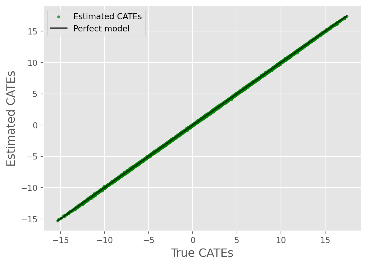
Let’s now look at the Precision in Estimating Heterogeneous Effects (PEHE) (e.g., RMSE) and plot some results for the treatment effects on each outcome:
from sklearn.metrics import root_mean_squared_error
from caml.extensions.plots import (
    cate_true_vs_estimated_plot,
    cate_histogram_plot,
    cate_line_plot,
)
true_cates1 = data_generator.cates.iloc[:, 0]
predicted_cates1 = cate_predictions[:, 0]
root_mean_squared_error(true_cates1, predicted_cates1)0.054197542640946cate_true_vs_estimated_plot(
true_cates=true_cates1, estimated_cates=predicted_cates1
)
cate_histogram_plot(true_cates=true_cates1, estimated_cates=predicted_cates1)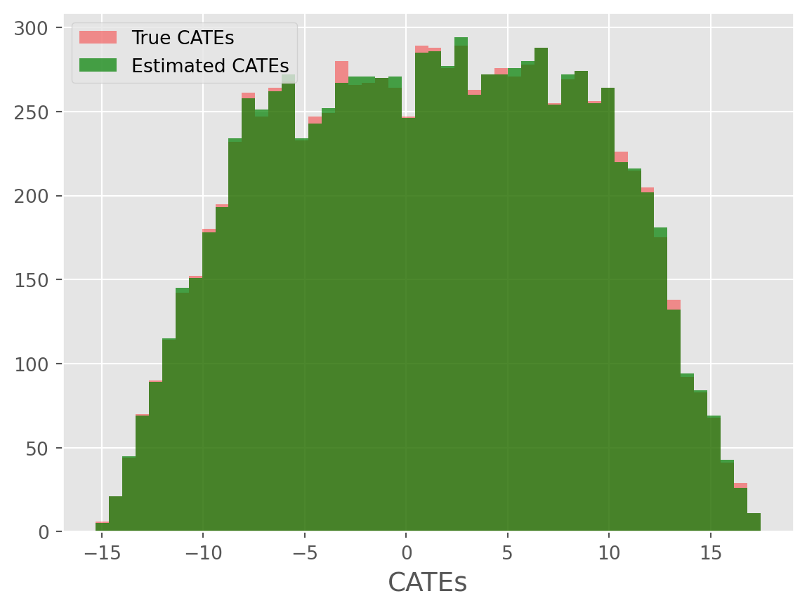
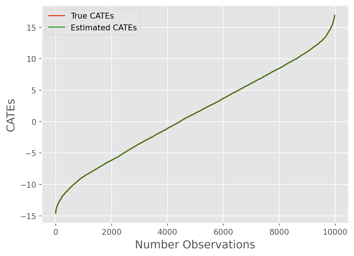
cate_line_plot(
    true_cates=true_cates1, estimated_cates=predicted_cates1, window=20
)
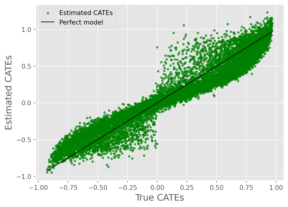
true_cates2 = data_generator.cates.iloc[:, 1]
predicted_cates2 = cate_predictions[:, 1]
root_mean_squared_error(true_cates2, predicted_cates2)0.15683038625127854cate_true_vs_estimated_plot(
true_cates=true_cates2, estimated_cates=predicted_cates2
)
cate_histogram_plot(true_cates=true_cates2, estimated_cates=predicted_cates2)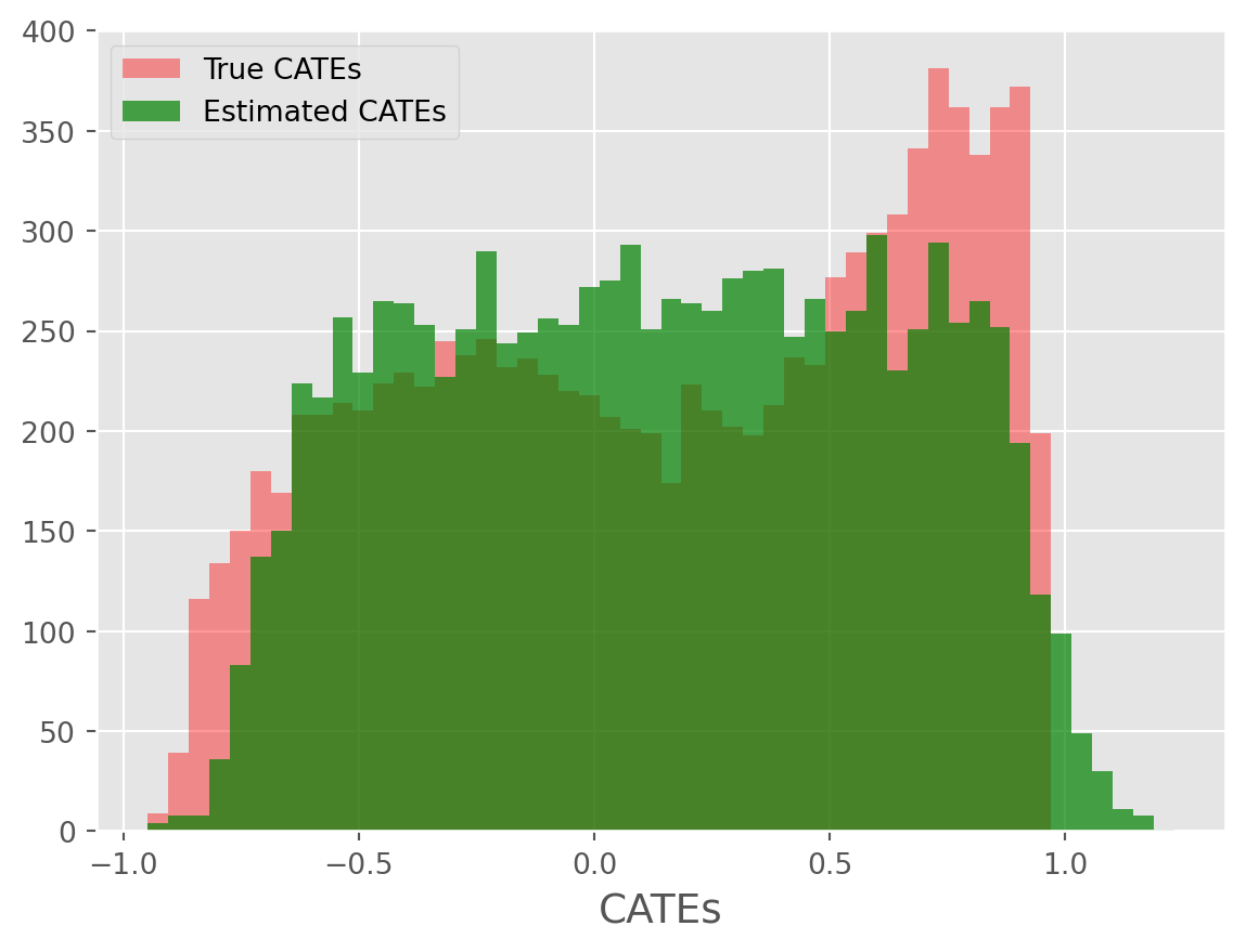
cate_line_plot(
    true_cates=true_cates2, estimated_cates=predicted_cates2, window=20
)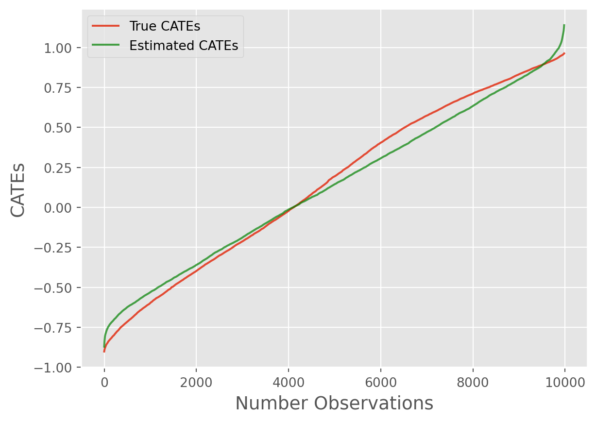
The CATE estimates for binary outcome using simulated data may perform poorly b/c of non-linear transformation (sigmoid) of linear logodds. In general, FastOLS should be prioritized when ATEs and GATEs are of primary interest. For high quality CATE estimation, we recommend leveraging CamlCATE.